MENU

SEA-XP Overview

SEA-XP Benefits

SEA-XP Theory

SEA-XP Toolbox

SEA-XP Specifications

SEA-XP Overview

SEA-XP is designed to provide all the tools needed to successfully acquire and process the data required to generate test-based simulation models. Some of the Features and Benefits of the software are:

Data Acquisition
SEA-XP offers a dedicated and portable data acquisition system. For added flexibility, SEA-XP also includes file format translators so that other data acquisition systems can be used.

SEA Parameter Computation
SEA parameters, DLF (Damping Loss Factors), CLF (Coupling Loss Factors) and modal density, are computed using different methods and with little operator’s input to avoid human errors in manipulating large amounts of data. This translates into reliable test-based models and a wealth of precious information for the refinement of SEA analytical models.

Decay Rate Estimation
SEA-XP’s signal processing capabilities make decay rate estimates quick and simple to perform, resulting in experimental data for acoustic absorption or structural damping. This feature offers a quick way to generate valuable input data for simulation models.

Much more...
Add variance analysis to assess data quality, extensive graphing and analysis features and flawless data transfer to theoretical SEA software.

SEA-XP Benefits

SEA-XP offers a hybrid approach to the prediction of noise and vibration by establishing a predictive model based on test data. More than just "test software", SEA-XP encourages synergy between test and simulation, essentially breaking down the traditional barrier between these methods.

SEA-XP processes experimental data to perform in-depth diagnosis and analysis of the broadband noise and vibration characteristics of your products. When used as a stand alone application, SEA-XP facilitates quality assessment on prototypes, resulting in more appropriate design modifications. Applied in conjunction with theoretical SEA software, SEA-XP facilitates the development of accurate and reliable simulated design models before a prototype is built.

In developing SEA-XP, our philosophy is to provide the noise and vibration engineer with all the tools needed to perform measurement and analysis on systems subjected to broadband excitation. As such, the SEA-XP toolbox is composed of three main modules: data acquisition, data processing and analysis.

Because a predictive model is derived from the test data, SEA-XP provides much more than "results from a test". Experimental SEA models are easily used to identify the dominant paths and sources in the system or to predict the behavior of the system when excitation conditions change. It is also possible to study the sensitivity of the solution to a certain parameter such as a DLF or CLF.

Test campaigns are often costly and result in a large amount of data that is difficult to properly review and exploit, especially at mid to high frequencies. SEA-XP reduces the data to a few key parameters, making it easy to access, comprehend and analyze for years to come.

Use SEA-XP in conjunction with theoretical SEA software such as SEA+ or SEAVirt Module to address all your predictive needs from mid to high frequencies. The comparison of measurement with prediction leads to refined models and ultimately saves time and reduces the risk of error. SEA-XP’s stand-alone capabilities are further enhanced by SEA+ and SEAVirt ability to simulate realistic design iterations.

In short, using SEA-XP along with SEA+ and SEAVirt, you develop a rigorous technology implementation program with a step-by-step approach, which guarantees the progressive development of more reliable and precise models. The reliance on testing is reduced as the program progresses towards the goal of full concept design prediction.

SEA-XP Theory

SEA-XP’s core technology is the implementation of the technique usually referred to as "Experimental SEA" (ESEA). In Statistical Energy Analysis (SEA), a matrix equation is solved to calculate the space average energy levels in the different parts of a structure (including its enclosed spaces). The ability for the energy to dissipate or propagate through the system is described by a matrix of loss factors L. This matrix is of dimension N×N where N is the number of substructures (called subsystems in the SEA terminology) that make up the system. A vector of power inputs {P} describes the mechanical and acoustic excitations to the system. The energy levels on the different subsystems are calculated for each frequency band of interest centered on w (w is expressed in radians). The matrix equation is written in collapsed form as:



The ESEA technique consists of inverting the process to calculate the parameters of the loss factor matrix from measurements of power and energy. These measurements are performed in a laboratory setting and require controlled excitation (such as impact hammer testing) to be applied to each subsystem in a sequential manner. For a system divided in N subsystems, there are N DLF (representing energy dissipation) and up to N(N − 1), CLF (representing energy transfer) to calculate. The N²×N² matrix that is solved is written in collapsed form as:



where the E_ij are the transfer energies between subsystems estimated from acceleration or acoustic pressure measurement. Once DLF and CLF are obtained, the equation can be applied to the prediction of energy levels in the measured system, and for a variety of input excitations.

SEA-XP Toolbox

SEA-XP includes a number of tools, some directly related to ESEA, some complementary. The tools available in the SEA-XP toolbox currently include:

Data acquisition of time histories and Frequency Response Functions (FRFs). The main advantages of using the SEA-XP built-in data acquisition system are:

• Portable PC-based system
• Data generated in SEA-XP format can be processed in real time

• Decay rate analysis which provides an alternative way of estimating damping
• Calculation of modes in band, which is very useful for comparison to analytical predictions
• User-defined analysis with formula builder working on multiple-file input
• File format translators for conversion of data acquired on a different system
• Time-frequency analysis

SEA-XP Specifications

Data Acquisition
Ready to use hardware solutions
SEA-XP may drive NI (National Instruments) based Data Acquisition cards for dynamic analysis.

Following configurations may be driven by SEA-XP under WINDOWS 7 to 10.

• Solution 1: Multiple-channels Acquisition on Notebook (16-bit resolution) with USB connection.
  
  NI USB acquisition using CompactRIO chassis with 1 to 4 NI 9234 4-channels acquisition module for a maximum of 16 channels, acquisition is synchroneous at 50 kHz and include on-board ICP signal conditioning.
  


• Solution 2: PXI acquisition using PXI or PXIe chassis with several plugged NI-44xx modules in order to perform multiple-channels 24 bits syncroneous acquisition on Desktop computer. Availble acquisition module are NI-4472 (8 channels 100 KHz/channel) and 4495 or 4496 (16 channels with 200 KHz/channel).

Acquisition Software Capabilities

Configurable number of channels when starting up the acquisition
Selection from 1 to the maximum supported by the board. Any NI card usable for analysis of dynamic signals may be used. For low-cost card with no hardware trigger, SEA-XP offers software trigger capability

Configurable sampling frequency
(the Max. frequency depend on hardware and on number of used channels in case of multiplexed boards)

Configurable record size for acquisition and FFT
From 128 points to 32768 points by step of 2

Continuous acquisition mode for random input
Transient recording on trigger for transient events
Configurable trigger
Setting of level, slope, time limit

Several modes available (depends on board) : software trigger mode (pre-trigger capabilities), hardware trigger mode (no pre-trigger), external TTL trigger

Quality Signal Detection (QSD)

Overload indication for all channels

Configurable low level detection for each recorded signals for safe detection of transducers that comes unstuck. Connected transducer but of which signal are not stored are not taken into account in Low level QSD

Powerful bounce detection for a constant impact hammer quality

During the averaging process all signals submitted to a positive QSD are rejected automatically from the average

Visual warning through LEDS on the front acquisition panel

Voice warning messages can be enabled (if a sound card is installed in the PC)

Signal Conditioner Control

SEA-XP can control a few number of older external signal conditioner connected to the RS-232 serial port of the PC motherboard. Gain and anti-aliasing filters (if any) of the conditioner are directly set from SEA-XP. A message is sent if no conditioner is detected

Present modern NI acquisition cards incorporates on-board ICP signal conditionning, controlled from the SEA-XP user-interface

Transducer Manager

SEA-XP handles a user’s defined transducer data base to quickly allocate a transducer to a given channel (ADD et SUPPRESS functions to manage the data base)

Auto-Calibration

User-defined calibrator frequency and level

Auto-calibration function for each channel when calibrator signal is applied

The calibration procedure is FFT based through the 1/rd octave filtering of the transducer response where the calibrator frequency is located. Calibration can then support noisy environment

Microphone Phase Correction (MPC) for Acoustic Intensity Measurement
SEA-XP incorporates Acoustic Intensity Measurement routines (see related topic). The MPC function allows to use two standard microphones to perform Acoustic Intensity

Interactive Control of external amplifier gain, internal card gain and transducer sensitivity
Storage of configuration setting, automatic retrieval of latest setting at start up

Data Signal Processing

Averaging Process

No average, Manual average, Auto-average (works under control of QSD), Auto-Average and store (works under control of QSD), when time data have been acquired

Interactive user definable number of averages (averaging process stops when the number is achieved), functions H1 and H2 available for FRF

Possibility to stop interactively an averaging process and to continue

Data Storage

Auto-Store (user definable): a selectable set of channels can be automatically stored with auto-indexing of records each time the acquisition is done. QSD function is used to control and prevent storage of bad data

Manual store, Works as previously except the "Store" button must pressed by the user

User definable storage of data type: for each channel selection between storage of either time history, autospectrum, FRF, QFRF, QFRF/Mobility

Visual indication of storing process (flashing LEDs, storage index)

Overwrite of stored data from a given storage index

Deletion of last stored sequence

Easy access to all stored data and files manipulation through the main user-interface of SEA-XP

Windowing

Rectangular

All Different

All the same:

- Same on first channel and second channel

- Same from second channel to end channel

User definable window selection

- Hanning, Hamming, Flat top, Blackman, Blackman-Harris, Exponential, Force…

- Interactive definition of window center and width

Acquisition Control

Detachable acquisition palette to command acquisition (storage, average, visualization, experiment progress, set parameters)

Background time history window : all time histories for all channels are visualized. A LED ramp for each channel indicates signal level

Zoom button: for each channel, open a window for real time processing of signal and zoom plot

Window button: for each channel, windowing of signal with a set of pre-defined window functions (see "Windowing")

Data type selector: user definable stored data type for each channel (see "Data Storage")

Oscilloscope mode: in continuous mode, plot windows are continuously refreshed. Zoom windows and background window are then working as a multi-channel oscilloscope

Real Time Signal Processing

In each zoom windows (several zoom windows can be open at the same time - one per channel only), a menu offers a choice of real time signal processing both in narrow band and 1/3rd octave band

Narrow Frequency Band Analysis

- Autospectrum

- Coherence

- FRF (frequency response function as zoomed channel / reference channel in transient recording mode, H1 or H2 in continuous recording mode)

- Q-FRF (quadratic frequency response function defined as locally frequency averaged zoom channel/ locally frequency averaged reference channel)

- Q-FRF/Mobility (locally frequency averaged zoom channel/ locally frequency averaged input mobility of the signal)

1/3rd octave frequency band analysis

Depending on transducer type allocated to the channel:

- RMS Sound pressure level spectrum

- RMS Force Spectrum

- RMS acceleration

- Real part of input mobility of zoomed channel/referenced channel

- RMS General value for undefined transducer

- FRF

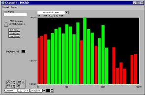
- Acoustic power

For Narrow Band and 1/3rd Octave

- Software DC filtering (on/off)

- Standard deviation of FFT analysis (in average mode)

Calibration Procedure

Called from zoom window

Visualization of Real Time Data

Access to data by

Zoom window

- Resizable

- 2D-Plot

- 3D WaterFall visualization for RMS spectra

- Graph zoom

- User definable x and y scale, Log, Lin

- Auto-scale (ON/OFF)

- Format and precision for scale labels

- Cursor (snap to point, free, Lock to point)

- Background color

- Information on signal

Visualization of Stored Data

Access to data by

Project Manager window: double click on file name

Preference menu to customize graphs

- 2D-multi plots

- Graph zoom

- User definable x and y scale, Log, Lin

- Auto-scale

- Format and precision for scale labels

- Cursor (snap to point, free, Lock to point)

- Background color, plot style

- Information on signal

- For complex signals : plot of real, imaginary part, phase and magnitude

- Niquyst plot

Store and Export from Zoom Window

Real time analysis in zoom window can be stored under SEA-XP or export to a file (spreadsheet format) or directly send to Excel under Active-X control. Data are automatically plot in Excel. Also available, Export to universal file format and export to picture (BMP format)

Print graph from zoom windows
The graph is directly sent to printer to be plotted

Copy&Paste Graph metafiles within Word or Excel

 

Experimental SEA Test Recording Facilities

Experimental SEA Test Definition in Project Manager
Test name, location, date, test specimen name, number of subsystems, subsystem names, user comments.

Experiment Progress Panel
SEA-XP implements 3 different protocols for experimental SEA. These protocols are selectable from the "Experiment Progress" panel. As soon as one protocol has been defined, the acquisition is automatically set to record the related measurement and help the user to follow the progress of the acquisition. This is particularly useful for FRF measurement as N² by the number of sampled points within a subsystem FRFs are needed to perform a complete SEA analysis. It can lead to huge database if N, number of subsystem is important. Up to 99 subsystems are available for analysis.

Implementation of Experimental SEA Test Protocols

FRF recording for velocity estimates, all SEA squared velocities and power results normalized by the autospectrum of the reference input

Q-FRF recording for velocity estimates, all SEA squared velocities and power normalized by the Q-autospectrum of the reference input

Q-FRF/Mobility all SEA squared velocities and power normalized by the real par of the input mobility

Auto-configuration of acquisition depending on test:
Reverberation time history

Power inject measurement

FRF measurement for further transfer velocity estimates

Q-FRF measurement for further transfer velocity estimates

FRF/Mobility

Matrix Visualization of FRF, Power Injected, Reverberation Time Recording

Auto Definition of Record Names

 

Direct to Disk Acquisition (Stream Acquisition)

Recording Functions

Stream to disk from 1 to all available channels. Performance depends on mounted board and PC hardware

Selectable sample frequency

Selectable number of streamed channels

Settings files compatible with the acquisition in record mode

Conditioner control under RS-232 setting

Auto-Range

Start up in manual mode or trigger mode, configurable stream time

Auto-store the already streamed data at any time on user command or on acquisition error

Real time visualization of recorded signal using decimated graphs

Storage of all channels in a binary .stream file

Post Visualization and Signal Processing of .Stream Files

Re-calibration function

Interactive visualization per block of 2n of each streamed channel

Animated graph and 3D-waterfall spectra

Pass band user definable Butterworth filtering and plot of time domain filtered data

Local RMS integration and plot of RMS time domain evolution

Interactive spectral density plot in either narrow band or 1/3rd octave

Animated spectral plots

Automatic analysis of multiple selection of stream files: store on output all 1/3rd spectral density files per user definable period of time to plot waterfall spectra

Statistics and Spectral Analysis

Statistic on user definable part of the signal: probability density, histogram, Min-Max level, % of time above a user definable threshold

Same functions on the absolute value of the time domain signal

Same functions on the rms. / time value of the time domain signal

dBA-weighting, linear and exponential average

Export Facilities

Export all signals to WAV format

Export current Graph to SEA-XP format for User’s define analysis

Export Mean autospectrum

Signal Test Generation

Generation of standard test signals (white, pink noise, windowed noise with Gaussian or Uniform probability density, sinus burst, sinus)

Export of test signals in WAV format to be played with a PC sound card

Project Manager

Project Manager Window
Easy access to all recorded data by selecting a test specimen to see all related records and by double clicking on file name to plot graphs

File manipulation: rename, suppress on multi file section

Data type filtering

Export facilities to Excel and TXT (spreadsheet format)

Direct import of TXT files in graphs

Project Manager menu
Access to all post-processing functions from the menu

Post-Processing Software Capabilities

Automatic ESEA Process

This is one of the most powerful features of SEA-XP. As soon as input data for ESEA are recorded, an automatic post-processing of all available data can be called.

During this post-processing, SEA-XP will reduce narrow band data to 1/3rd octave spaced and frequency averaged spectrum per subsystem, will derive from FRF the average reverberation time of individual subsystems in order to automatically generate the equivalent masses of all subsystems. At the end the complete model is constructed and plot within the graphic window of the Experimental SEA. solver.

Automatic generation of input power vector from time decay if measured power not available.

In case you want to get a personal feeling on this background post-processing, manual post-processing of individual data is possible using hereafter described functions.

Experimental Injected Power

Input Data:

Force and acceleration time history at input point, or

Input point complex FRF

Auto-selection of inputs from file name and subsystem number or user definable through multiple file selection

Output:

Complex Mobility or Injected Power

Coherence

Experimental negative values filtering

Sign change

Standard deviation

Narrow frequency band outputs in ASCII or binary format and 1/3 octave frequency band outputs

Experimental 1/3 Octave Mean Velocity

Input Data:

FRF, Q-FRF or Q-FRF Mobility

Output:

1/3rd octave averaged per subsystem quadratic velocity

Automatic compacting per subsystem

Standard deviations of both point to point velocity and spaced averaged velocity

Selection of coupling to be neglected

Decay Rate and Related Functions

Experimental Reverberation Time

Input data: multiple selection of FRFs or time histories 1/Nth. octave selectable high order Butterworth filtering of time histories, Hilbert envelope, Schroeder smoothing options, equivalent mass correction

Outputs: reverberation time, DLF in 1/Nth octave band

Automatic interpolation from 1/Nth to 1/3rd octave

Automatic computation mode (automatic average with multi-file input)

In manual mode

Interactive reverberation time (RT) graphical determination

Interactive standard deviation

Interactive data smoothing

Visualization of synthesized impulse response and filtered impulse response

Absorption Coefficient Computation

Conversion of reverberation time into Absorption coefficient from user definable acoustic volume properties

Experimental Equivalent Mass

Compute equivalent mass for a subsystem from reverberation time, injected power and average velocity

Input Power from Decay Rate

Generate input power from reverberation time and average velocity for a given subsystem for both structural and acoustical subsystems

Transmission Loss

Compute the room transmission loss coefficient from pressure signals of emitter and receiver

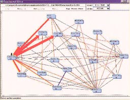
Experimental SEA

ESEA model managing in 2D-user’s graphical interface
Iconic user definable representation of subsystems in the 2D network

Graphical setting of coupling between subsystems through 2D-network connectors or matrix view

Storage of model and results in a compact binary file

Subsystem compacting

To derive simpler sub-structuring from an original model include:

Subsystem suppression

Subsystem union

Automatic renumbering of subsystems

"Connect All" function available

CLF, DLF identification

Use selectable frequency dependent equivalent mass or user definable mass

Ø Ø Ø CLF, DLF computation, from database of power, equivalent mass and transfer velocity’s

- Use Random Monte-Carlo matrix inversion to estimate DLF and CLF stability

- SVD algorithm and solution through matrix pseudo inverse

- Filtering of positive solutions with different probability law simulation

- Simplify CLF computation available

- CLF and DLF standard deviation computation

- Import CLF or DLF or any parameters from other models including coupling scheme

Interactive Visualization of experimental power flow, synthesized power flow, computation of synthesized energy, plot of power inputs and power losses plots for each subsystem

Diagnosis Tool

For a better understanding of complex systems

- Sort subsystems relatively to coherence, standard deviation

- Easy and quick way to suppress not valid FRF measurements

Extra Parameters

Experimental modal density

Compute modes/Hz and the number of modes / 1/3 octave from power measurements.

Modal overlap plot

Source Power Identification

Compute input power vector from an ESEA loss factor matrix and the average velocity vector estimated in working condition using Random Monte Carlo procedure

Power Standard Deviation Estimation

1/3 octave averaged spectral power density.
Automatic processing of groups of acceleration, force or acoustic signals

1/3 octave or narrow frequency band signal re-calibration possible

All Outputs in VAONE compatible units

File Computation Utility

Use graphical formulas that operate on multi-file selections or internally generated signals

Operators:

Add, subtract, multiply, divide, squared, square root

Min, max,

SIN, COS, TAN

20Log, 10Log, Log, 10^

Module, Re, Im, Phase

Arithmetic mean

Geometric mean

Weighting mean

File summation, integration, derivation

Standard deviation

RMS

FFT Spectrum

Hilbert envelope

Generate signal: sine, cosine, triangle, square, saw tooth, ramp (increasing or decreasing), user definable through interactive text formula

Time / Frequency Analysis

Input files : FRF or time history

Method: Short termed FFT, Wigner-Ville transform

Using Wigner-Ville (WV):

For a single input signal WV autospectrum / time

For two input signals: WV cross-spectrum, cross-spectrum mobility, injected power, injected power mobility

Selectable Window size for analysis and windows type (Rectangular, Hanning…)

Analysis can be performed on a selected part of the signal

Smooth parameters available (pseudo-WV)

Memory consumption tracking prior to computation to avoid hard disk swap

External Interface

Export all 1/3 octave files to Dataset 58 (universal txt format) for import in theoretical SEA software (SEA+ or other) in Universal File Format

Conversion of Universal files and ASCII files to SEA-XP binary files

Write to Universal File Format from Graph windows

Back to top